![]()
Contents |
 |
![]()
Self-organizing maps - also called Kohonen feature maps - are a special kind of neural networks that can be used for clustering tasks. They are an extension of the so-called learning vector quantization. Note, however, that this document cannot provide an exhaustive explanation of self-organizing maps (see any textbook on neural networks for that). Rather, it only briefly recalls the basic ideas underlying this kind of neural networks.
A self-organizing map consists of two layers of neurons: an input layer and a so-called competition layer. The weights of the connections from the input neurons to a single neuron in the competition layer are interpreted as a reference vector in the input space. That is, a self-organizing map basically represents a set of vectors in the input space: one vector for each neuron in the competition layer.
A self-organizing map is trained with a method that is called competition learning: When an input pattern is presented to the network, that neuron in the competition layer is determined, the reference vector of which is closest to the input pattern. This neuron is called the winner neuron and it is the focal point of the weight changes. In pure competition learning - as it is used in learning vector quantization - only the weights of the connections leading to the winner neuron are changed. The changes are made in such a way that the reference vector represented by these weights is moved closer to the input pattern.
In self-organizing maps, however, not only the weights of the connections to the winner neuron are adapted. Rather, there is a neighborhood relation defined on the competition layer which indicates which weights of other neurons should also be changed. This neighborhood relation is usually represented as a (usually two-dimensional) grid, the vertices of which are the neurons. This grid most often is rectangular or hexagonal. During the learning process, the weights of all neurons in the competition layer that lie within a certain radius around the winner neuron w.r.t. this grid are also adapted, although the strength of the adaption may depend on their distance from the winner neuron.
The effect of this learning method is that the grid, by which the neighborhood relation on the competition layer is defined, is "spread out" over the region of the input space that is covered by the training patterns. The programs xsom and wsom visualize this process for a very simple learning task.
| back to the top |  |
![]()
The training process of a self-organizing map can easily be visualized if we use a simple learning problem, namely the problem to cover a certain two-dimensional region with a rectangular grid of neurons. To keep things simple, the programs xsom and wsom consider only a square region, a triangular region, or a circular region. To be more specific, all of these regions are located around the origin of a two-dimensional coordinate system and extend from -1 to 1 in both dimensions.
At the beginning of the training process the weights of the connections from the input layer to the competition layer are initialized with random values from a certain interval. Then random patterns are generated, which are uniformly distributed over the chosen region. For each pattern the winner neuron is determined and the weights of the connections to this neuron and to its neighboring neurons are adapted. In the course of time the learning rate (i.e., the severity of the weight changes) as well as the neighborhood radius (and thus the set of neurons that are adapted apart from the winner neuron) is reduced. Finally the network reaches a more or less stable state, in which the weight changes almost cease.
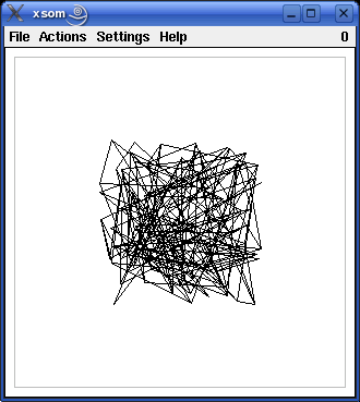
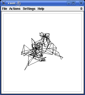
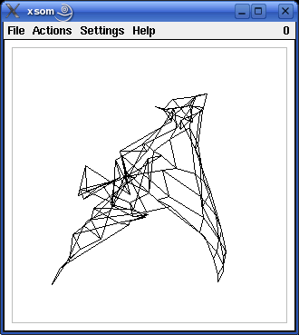
An example of the development of a self-organizing map, as it can be observed with the programs xsom and wsom, is shown in the screenshots below. The window shows the input space of the self-organizing map. The training pattern region, which in this case is the square [-1,1]x[-1,1], is indicated by grey lines in the screenshots. The black lines show the grid of the competition layer of the self-organizing map as it is mapped to the input space.
The upper left screenshot shows the situation after the random initialization. Each corner point, i.e., each point where black lines meet, represents a reference vector, i.e., a neuron of the competition layer. The lines connect neurons w.r.t. the grid that defines the neighborhood relation on the competition layer. However, since the weights are initialized randomly, this grid is not discernable at this point.
The following screenshots (proceeding from left to right and from top to bottom) show the self-organizing map after 10, 20, 40, 80 and 160 steps (training patterns). As the training proceeds, the grid structure, in which the neurons are organized, becomes more and more visible. Finally, the grid has unfolded completely and covers the training pattern region fairly well.
 |
 |
 |
 |
 |
 |
(Exercise: Why is there always a gap between the grid representing the self-organizing map and the border of the training pattern region?)
This example was produced with the default parameters: The competition layer is a rectangular grid of 10x10 neurons. The weights were initialized with random values between -0.5 and 0.5. The learning rate was computed according to the formula eta(t) = 0.6 t-0.1, the neighborhood radius according to the formula r(t) = 2.5 t-0.1. In both formulae t is the time, which is measured by the number of processed training patterns. The unit of the neighborhood radius is the grid width (see also the "parameters" section below).
However, the default parameters are not optimal for the default size of the map (i.e., 10x10 neurons). In particular, the value of the neighborhood radius is somewhat too small. As a consequence the map sometimes becomes twisted (see the screenshot below). Such twisted maps are, of course, undesirable. They can almost surely be avoided by using a larger initial radius (e.g. r0 = 9), which (to compensate for the larger radius) is decreased at a faster pace (e.g. radius decay exponent kr = 0.3). Another reason for a twisted map may be that the learning rate was chosen too low.
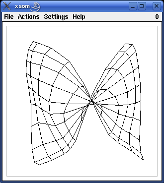
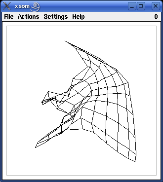
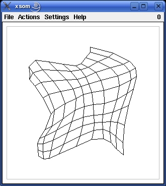
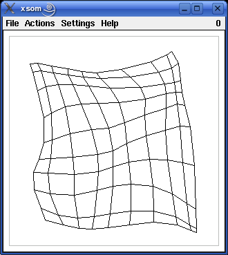
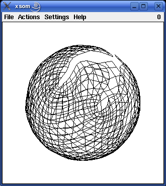
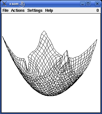
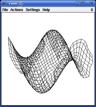
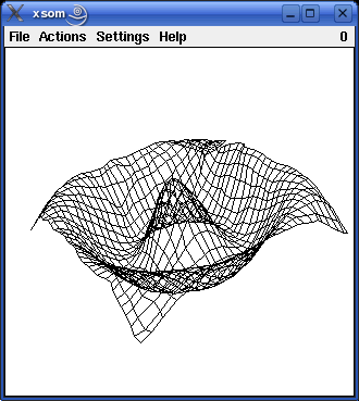
Since version 2.0 the programs also visualize training a self-organizing map for three-dimensional input data. There are four three-dimensional pattern regions to choose from: the surface of a sphere, a rotated parabola, a cubic function and a cosine function. These three-dimensional pattern regions may be somewhat better suited to demonstrate the idea of self-organizing maps, because people tend to be confused by the fact that for the other three example the input space and the map have the same number of dimensions. The following pictures show self-organizing maps with 30x30 neurons for the four different three-dimensional pattern regions. (Gaussian neighborhood, initial neighborhood radius 30, radius decay exponent 0.4, trained with about 10000 patterns.)
 |
 |
 |
 |
The three-dimensional maps can be rotated by moving the mouse with the left or the middle mouse button pressed. They can be zoomed by moving the mouse with the right mouse button pressed.
| back to the top |  |
![]()
If the menu entry Settings > Grid/Shape... is selected (or, in the Unix version, if `g' for `grid' is pressed), a dialog box is opened in which the shape of the pattern region and the dimensions of the grid of the competition layer of the self-organizing map may be entered (this dialog box is shown below).
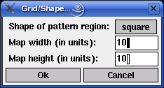
Possible shapes of the pattern region are `square' (this is the default), `triangle', `circle', `sphere', `parabola', `cubic', and `cosine'. With these shapes it can be demonstrated how a self-organizing map adapts to the different sets of training patterns. The last four choices are three-dimensional pattern regions, but can be fitted well with a two-dimensional map.
The competition layer of the self-organizing map used by the programs has a square/rectangular grid. Each grid point corresponds to one neuron. Hence the competition layer can be specified completely by stating the width and the height of this grid. The default is 10x10 neurons. The maximum size is 100x100 neurons.
The learning process of the self-organizing map is influenced by several parameters. If the menu entry Settings > Parameters... is selected (or, in the Unix version, if `p' for `parameters' is pressed), a dialog box is opened in which these parameters can be changed (this dialog box is shown below).
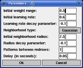
| Initial weight range: | At the beginning of the training process, the weights of the self-organizing map are chosen randomly from the interval [-x,x]. In this field the value of x may be entered. The default is 0.5. | |
| Initial learning rate: | The learning rate is decreased with time according to the formula eta(t) = eta0tketa (if keta is negative) or according to the formula eta(t) = eta0ketat (if keta is positive). Here t is the time, which is measured as the number of processed training patterns. In this field the value of the initial learning rate eta0 may be entered. The default is 0.6, which means that for the first training pattern the reference vector of the winner neuron is moved 0.6 of its (Euclidean) distance from the training pattern towards this training pattern. | |
| Learning rate decay exponent: | In this field the value of the decay parameter keta may be entered (cf. the description of the preceding field). The default is -0.1. | |
| Neighborhood type: | Either `rectangular' or `Gaussian'. If the type is `rectangular', all neurons within the current neighborhood radius (Euclidean distance w.r.t. the grid of the competition layer) around the winner neuron are adapted with the same strength as the winner neuron, whereas all neurons outside this radius are not adapted. That is, a rectangular neighborhood function is used. If the type is `Gaussian', all neurons are adapted, but with a strength that is computed from a Gaussian function that is normalized to maximum 1 and is centered at the winner neuron. In this case the neighborhood radius is the `standard deviation' of the Gaussian function. Usually a Gaussian neighborhood leads to smoother training behavior, therefore it is the default. | |
| Initial neighborhood radius: | Like the learning rate, the neighborhood radius is decreased with time according to the formula r(t) = r0tkr (if kr is negative) or according to the formula r(t) = r0krt (if kr is positive). Here t is the time, which is measured as the number of processed training patterns. The unit of the radius is the width of the grid that defines the neighborhood of the neurons in the competition layer. In this field the value of the initial neighborhood radius r0 may be entered. The default is 2.5. | |
| Radius decay exponent: | In this field the value of the decay exponent kr may be entered (cf. the description of the preceding field). The default is -0.1. | |
| Epochs between redraws: | Since processing one training pattern often does not produce a considerable change of the map, several training steps may be performed before the map is redrawn. In this field this number of patterns may be entered. The default is 1, i.e., the map is redrawn after each training pattern. | |
| Delay: | The time between two consecutive training steps. By enlarging this value the training process can be slowed down or even executed in single steps. The default is 0.05 seconds. |
All entered values are checked for plausibility. If a value is entered that lies outside the acceptable range for the parameter (for example, a negative learning rate), it is automatically corrected to the closest acceptable value.
A self-organizing map can also be saved to a file and reloaded later. To do so one has to select the menu entries File > Save Map... or File > Load Map..., respectively. (Alternatively, in the Unix version, one may press `s' for `save' and `l' for `load'.) The file selector box that is opened, if one of these menu entries are selected, is shown below. (In the Windows version the standard Windows file selector box is used.)
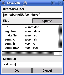
The edit field below 'Directory/Filter' shows the current path, the list box below 'Files' the files in the current directory matching the current file name pattern. (A file name pattern, which may contain the usual wildcards '*' and '?', may be added to the path. When the file name pattern has been changed, pressing the 'Update' button updates the file list.) The line below 'Selection' shows the currently selected file. It may be chosen from the file list or typed in.
| back to the top |  |
![]()
(MIT license, or more precisely Expat License; to be found in the file mit-license.txt in the directory somd/doc in the source package, see also opensource.org and wikipedia.org)
© 2000-2016 Christian Borgelt
Permission is hereby granted, free of charge, to any person obtaining a copy of this software and associated documentation files (the "Software"), to deal in the Software without restriction, including without limitation the rights to use, copy, modify, merge, publish, distribute, sublicense, and/or sell copies of the Software, and to permit persons to whom the Software is furnished to do so, subject to the following conditions:
The above copyright notice and this permission notice shall be included in all copies or substantial portions of the Software.
THE SOFTWARE IS PROVIDED "AS IS", WITHOUT WARRANTY OF ANY KIND, EXPRESS OR IMPLIED, INCLUDING BUT NOT LIMITED TO THE WARRANTIES OF MERCHANTABILITY, FITNESS FOR A PARTICULAR PURPOSE AND NONINFRINGEMENT. IN NO EVENT SHALL THE AUTHORS OR COPYRIGHT HOLDERS BE LIABLE FOR ANY CLAIM, DAMAGES OR OTHER LIABILITY, WHETHER IN AN ACTION OF CONTRACT, TORT OR OTHERWISE, ARISING FROM, OUT OF OR IN CONNECTION WITH THE SOFTWARE OR THE USE OR OTHER DEALINGS IN THE SOFTWARE.
| back to the top |  |
![]()
Download page with most recent version.
| back to the top |  |
![]()
| E-mail: |
christian@borgelt.net | |
| Website: |
www.borgelt.net |
| back to the top |  |
![]()